Introducing read_waterdata_samples
Laura A. DeCicco
Source:vignettes/samples_data.Rmd
samples_data.RmdAs we bid adieu to the NWIS discrete water quality services, we welcome a new web service offering, the U.S. Geological Survey (USGS) Water Data for the Nation samples data service.
In this tutorial, we’ll walk through how to use the new services in the following ways:
Retrieving data from a known USGS site.
Retrieving data using different geographical filters.
Discovering available data.
For more information on the new data formats, see: https://waterdata.usgs.gov/blog/qw-to-wqx3-mapping
New USGS data access
This is a modern access point for USGS discrete water quality data.
The USGS is planning to modernize all web services in the near future.
For each of these updates, dataRetrieval will create a new
function to access the new services. To access these services on a web
browser, go to https://waterdata.usgs.gov/download-samples/.
New Features
Style
New functions will use a “snake case”, such as “read_waterdata_samples”. Older functions use camel case, such as “readNWISdv”. The difference is the underscore between words. This should be a handy way to tell the difference between newer modern data access, and the older traditional functions.
Structure
Historically, we allowed users to customize their queries via the
... argument structure. With ..., users needed
to know the exact names of query parameters before using the function.
Now, the new functions will include ALL possible
arguments that the web service APIs support. This will allow users to
use tab-autocompletes (available in RStudio and other IDEs).
Users will need to understand that it is not advisable to
specify all of these parameters. The systems can get bogged down with
redundant query parameters. We expect this will be easier for
users, but it might take some time to smooth out the documentation and
test usability. There may be additional consequences, such as users
won’t be able to build up argument lists to pass into the function.
Discrete USGS data workflow
Alright, let’s test out this new service! Here is a link to the user interface: https://waterdata.usgs.gov/download-samples.
And here is a link to the web service documentation: https://api.waterdata.usgs.gov/samples-data/docs
Retrieving data from a known site
Let’s say we have a USGS site. We can check the data available at
that site using summarize_waterdata_samples like this:
library(dataRetrieval)
site <- "USGS-04183500"

data_at_site <- summarize_waterdata_samples(monitoringLocationIdentifier = site)
## GET: https://api.waterdata.usgs.gov/samples-data/summary/USGS-04183500?mimeType=text%2FcsvExplore the results:
We see there’s 1288 filtered phosphorus values available. Note that if we ask for a simple characteristic = “Phosphorus”, we’d get back both filtered and unfiltered, which might not be appropriate to mix together in an analysis. “characteristicUserSupplied” allows us to query by a very specific set of data. It is similar to a long-form USGS parameter code.
To get that data, use the read_waterdata_samples
function:
user_char <- "Phosphorus as phosphorus, water, unfiltered"
phos_data <- read_waterdata_samples(monitoringLocationIdentifier = site,
                        characteristicUserSupplied = user_char)
## No profile specified, defaulting to 'fullphyschem'
## Possible values are:
## fullphyschem, basicphyschem, fullbio, basicbio, narrow, resultdetectionquantitationlimit, labsampleprep, count## GET: https://api.waterdata.usgs.gov/samples-data/results/fullphyschem?mimeType=text%2Fcsv&monitoringLocationIdentifier=USGS-04183500&characteristicUserSupplied=Phosphorus%20as%20phosphorus%2C%20water%2C%20unfilteredInspecting phos_data, there are 193 columns (!). That is because the default dataProfile is “Full physical chemical”, which is designed to be comprehensive.
Instead of using the “Full physical chemical” profile, we could ask for the “Narrow” profile, which contains fewer columns:
phos_narrow <- read_waterdata_samples(monitoringLocationIdentifier = site,
                        characteristicUserSupplied = user_char,
                        dataProfile = "narrow")
## GET: https://api.waterdata.usgs.gov/samples-data/results/narrow?mimeType=text%2Fcsv&monitoringLocationIdentifier=USGS-04183500&characteristicUserSupplied=Phosphorus%20as%20phosphorus%2C%20water%2C%20unfilteredWe can do a simple plot to check the data:
library(ggplot2)
wrap_text <- function(x, width = 30, collapse = "\n"){
  new_text <- paste(strwrap(x,
                width = width),
                collapse = collapse)
  return(new_text)
}

ggplot(data = phos_narrow) +
  geom_point(aes(x = Activity_StartDateTime,
                 y = Result_Measure)) +
  theme_bw() +
  ggtitle(unique(phos_narrow$Location_Name)) +
  xlab("Date") +
  ylab(wrap_text(unique(phos_narrow$Result_CharacteristicUserSupplied)))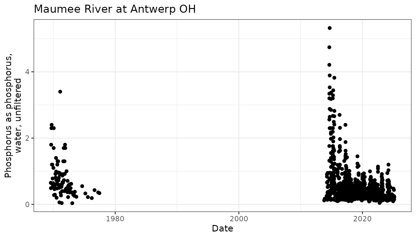
Return data types
There are 2 arguments that dictate what kind of data is returned: dataType and dataProfile. The “dataType” argument defines what kind of data comes back, and the “dataProfile” defines what columns from that type come back.
The possibilities are (which match the documentation here):
- dataType = “results”
- dataProfile: “fullphyschem”, “basicphyschem”, “fullbio”, “basicbio”, “narrow”, “resultdetectionquantitationlimit”, “labsampleprep”, “count”
- dataType = “locations”
- dataProfile: “site”, “count”
- dataType = “activities”
- dataProfile: “sampact”, “actmetric”, “actgroup”, “count”
- dataType = “Projects”
- dataProfile: “project”, “projectmonitoringlocationweight”
- dataType = “organizations”
- dataProfile: “organization” and “count”
Geographical filters
Let’s say we don’t know a USGS site number, but we do have an area of interest. Here are the different geographic filters available. We’ll use characteristicUserSupplied = “Phosphorus as phosphorus, water, unfiltered” to limit the sites returned, and dataType = “locations” to limit the data returned. That means we’ll just be asking for what sites measured “Phosphorus as phosphorus, water, unfiltered”, but not actually getting those result values.
Bounding Box
North and south are latitude values; east and west are longitude values. A vector of 4 (west, south, east, north) is expected.
bbox <- c(-90.8, 44.2, -89.9, 45.0)
user_char <- "Phosphorus as phosphorus, water, unfiltered"

bbox_sites <- read_waterdata_samples(boundingBox = bbox,
                                characteristicUserSupplied = user_char,
                                dataType = "locations",
                                dataProfile = "site")
Hydrologic Unit Codes (HUCs)
Hydrologic Unit Codes (HUCs) identify physical areas within the US that drain to a certain portion of the stream network. This filter accepts values containing 2, 4, 6, 8, 10 or 12 digits.
huc_sites <- read_waterdata_samples(hydrologicUnit = "070700",
                                characteristicUserSupplied = user_char,
                                dataType = "locations",
                                dataProfile = "site")
## GET: https://api.waterdata.usgs.gov/samples-data/locations/site?mimeType=text%2Fcsv&hydrologicUnit=070700&characteristicUserSupplied=Phosphorus%20as%20phosphorus%2C%20water%2C%20unfilteredDistance from a point
Location latitude (pointLocationLatitude) and longitude (pointLocationLongitude), and the radius (pointLocationWithinMiles) are required for this geographic filter:
point_sites <- read_waterdata_samples(pointLocationLatitude = 43.074680,
                                 pointLocationLongitude = -89.428054,
                                 pointLocationWithinMiles = 20,
                                characteristicUserSupplied = user_char,
                                dataType = "locations",
                                dataProfile = "site")
## GET: https://api.waterdata.usgs.gov/samples-data/locations/site?mimeType=text%2Fcsv&characteristicUserSupplied=Phosphorus%20as%20phosphorus%2C%20water%2C%20unfiltered&pointLocationLatitude=43.07468&pointLocationLongitude=-89.42805&pointLocationWithinMiles=20countyFips
County query parameter. To get a list of available counties, run
check_waterdata_sample_params("counties"). The “Fips”
values can be created using the function
countyCdLookup.
dane_county <- countyCdLookup("WI", "Dane",
                              outputType = "fips")
## GET: https://api.waterdata.usgs.gov/samples-data/codeservice/counties?mimeType=application%2Fjson## GET: https://api.waterdata.usgs.gov/samples-data/codeservice/states?mimeType=application%2Fjson
## GET: https://api.waterdata.usgs.gov/samples-data/codeservice/states?mimeType=application%2Fjson
county_sites <- read_waterdata_samples(countyFips = dane_county,
                                characteristicUserSupplied = user_char,
                                dataType = "locations",
                                dataProfile = "site")
## GET: https://api.waterdata.usgs.gov/samples-data/codeservice/states?mimeType=application%2Fjson## GET: https://api.waterdata.usgs.gov/samples-data/codeservice/counties?mimeType=application%2Fjson## GET: https://api.waterdata.usgs.gov/samples-data/locations/site?mimeType=text%2Fcsv&characteristicUserSupplied=Phosphorus%20as%20phosphorus%2C%20water%2C%20unfiltered&countyFips=US%3A55%3A025stateFips
State query parameter. To get a list of available state fips values,
run check_waterdata_sample_params("states"). The “fips”
values can be created using the function stateCdLookup.
state_fip <- stateCdLookup("WI", outputType = "fips")## GET: https://api.waterdata.usgs.gov/samples-data/codeservice/states?mimeType=application%2Fjson
state_sites <- read_waterdata_samples(stateFips = state_fip,
                                characteristicUserSupplied = user_char,
                                dataType = "locations",
                                dataProfile = "site")
## GET: https://api.waterdata.usgs.gov/samples-data/codeservice/states?mimeType=application%2Fjson## GET: https://api.waterdata.usgs.gov/samples-data/locations/site?mimeType=text%2Fcsv&characteristicUserSupplied=Phosphorus%20as%20phosphorus%2C%20water%2C%20unfiltered&stateFips=US%3A55Additional Query Parameters
Additional parameters can be included to limit the results coming back from a request.
siteTypeCode
Site type code query parameter.
site_type_info <- check_waterdata_sample_params("sitetype")## GET: https://api.waterdata.usgs.gov/samples-data/codeservice/sitetype?mimeType=application%2Fjson
site_type_info$typeCode## [1] "GL" "WE" "LA" "LA-EX"
## [5] "LA-OU" "LA-PLY" "LA-SNK" "LA-SH"
## [9] "LA-SR" "LA-VOL" "AT" "ES"
## [13] "OC" "OC-CO" "LK" "ST"
## [17] "ST-CA" "ST-DCH" "ST-TS" "SP"
## [21] "GW" "GW-CR" "GW-EX" "GW-HZ"
## [25] "GW-IW" "GW-MW" "GW-TH" "SB"
## [29] "SB-CV" "SB-GWD" "SB-TSM" "SB-UZ"
## [33] "FA" "FA-AWL" "FA-CI" "FA-CS"
## [37] "FA-DV" "FA-FON" "FA-GC" "FA-HP"
## [41] "FA-QC" "FA-LF" "FA-OF" "FA-PV"
## [45] "FA-SPS" "FA-STS" "FA-TEP" "FA-WIW"
## [49] "FA-SEW" "FA-WWD" "FA-WWTP" "FA-WDS"
## [53] "FA-WTP" "FA-WU" "AG" "AS"
## [57] "AW" "SS"siteTypeName
Site type name query parameter.
site_type_info$typeLongName## [1] "Glacier"
## [2] "Wetland"
## [3] "Land"
## [4] "Excavation"
## [5] "Outcrop"
## [6] "Playa"
## [7] "Sinkhole"
## [8] "Soil hole"
## [9] "Shore"
## [10] "Volcanic vent"
## [11] "Atmosphere"
## [12] "Estuary"
## [13] "Ocean"
## [14] "Coastal"
## [15] "Lake, Reservoir, Impoundment"
## [16] "Stream"
## [17] "Canal"
## [18] "Ditch"
## [19] "Tidal stream"
## [20] "Spring"
## [21] "Well"
## [22] "Collector or Ranney type well"
## [23] "Extensometer well"
## [24] "Hyporheic-zone well"
## [25] "Interconnected wells"
## [26] "Multiple wells"
## [27] "Test hole not completed as a well"
## [28] "Subsurface"
## [29] "Cave"
## [30] "Groundwater drain"
## [31] "Tunnel, shaft, or mine"
## [32] "Unsaturated zone"
## [33] "Facility"
## [34] "Animal waste lagoon"
## [35] "Cistern"
## [36] "Combined sewer"
## [37] "Diversion"
## [38] "Field, Pasture, Orchard, or Nursery"
## [39] "Golf course"
## [40] "Hydroelectric plant"
## [41] "Laboratory or sample-preparation area"
## [42] "Landfill"
## [43] "Outfall"
## [44] "Pavement"
## [45] "Septic system"
## [46] "Storm sewer"
## [47] "Thermoelectric plant"
## [48] "Waste injection well"
## [49] "Wastewater sewer"
## [50] "Wastewater land application"
## [51] "Wastewater-treatment plant"
## [52] "Water-distribution system"
## [53] "Water-supply treatment plant"
## [54] "Water-use establishment"
## [55] "Aggregate groundwater use"
## [56] "Aggregate surface-water-use"
## [57] "Aggregate water-use establishment"
## [58] "Specific Source"activityMediaName
Sample media refers to the environmental medium that was sampled or analyzed.
media_info <- check_waterdata_sample_params("samplemedia")## GET: https://api.waterdata.usgs.gov/samples-data/codeservice/samplemedia?mimeType=application%2Fjson
media_info$activityMedia## [1] "Air" "Biological tissue"
## [3] "Other" "Sediment"
## [5] "Soil" "Water"
## [7] NAcharacteristicGroup
Characteristic group is a broad category describing the sample measurement. The options for this parameter generally follow the values described in the Water Quality Portal User Guide, but not always.
group_info <- check_waterdata_sample_params("characteristicgroup")## GET: https://api.waterdata.usgs.gov/samples-data/codeservice/characteristicgroup?mimeType=application%2Fjson
group_info$characteristicGroup## [1] "Biological"
## [2] "Information"
## [3] "Inorganics, Major, Metals"
## [4] "Inorganics, Major, Non-metals"
## [5] "Inorganics, Minor, Metals"
## [6] "Inorganics, Minor, Non-metals"
## [7] "Microbiological"
## [8] "Nutrient"
## [9] "Organics, Other"
## [10] "Organics, PCBs"
## [11] "Organics, Pesticide"
## [12] "Organics, PFAS"
## [13] "Physical"
## [14] "Population/Community"
## [15] "Radiochemical"
## [16] "Sediment"
## [17] "Stable Isotopes"
## [18] "Toxicity"characteristic
Characteristic is a specific category describing the sample. See
check_waterdata_sample_params("characteristics") for a full
list, below is a small sample:
characteristic_info <- check_waterdata_sample_params("characteristics")## GET: https://api.waterdata.usgs.gov/samples-data/codeservice/characteristics?mimeType=application%2Fjson## [1] "Hydroxy-amitriptyline, 10-"
## [2] "1,1,1,2-Tetrachloroethane"
## [3] "1,1,1-Trichloro-2-propanone"
## [4] "1,1,1-Trichloroethane"
## [5] "1,1,2,2-Tetrachloroethane"
## [6] "CFC-113"characteristicUserSupplied
Observed property is the USGS term for the constituent sampled and
the property name gives a detailed description of what was sampled.
Observed Property is mapped to characteristicUserSupplied, and replaces
the parameter name and pcode USGS previously used to describe discrete
sample data. See
check_waterdata_sample_params("observedproperty") for a
full list, below is a small sample:
char_us <- check_waterdata_sample_params("observedproperty")## GET: https://api.waterdata.usgs.gov/samples-data/codeservice/observedproperty?mimeType=application%2Fjson
head(char_us$observedProperty)## [1] "10-Hydroxy-amitriptyline, water, filtered, recoverable"
## [2] "1,1,1,2-Tetrachloroethane, bed sediment (dry mass basis), recoverable"
## [3] "1,1,1,2-Tetrachloroethane, soil (dry mass basis), recoverable"
## [4] "1,1,1,2-Tetrachloroethane, water, unfiltered, recoverable"
## [5] "1,1,1-Trichloro-2-propanone, water, filtered, recoverable"
## [6] "1,1,1-Trichloro-2-propanone, water, unfiltered, EPA method 551.1"usgsPCode
USGS parameter code. See
check_waterdata_sample_params("characteristics") for a full
list, below is a small sample:
characteristic_info <- check_waterdata_sample_params("characteristics")## GET: https://api.waterdata.usgs.gov/samples-data/codeservice/characteristics?mimeType=application%2Fjson## [1] "67995" "52417" "62235" "30089" "77562"
## [6] "51330"projectIdentifier:
Project identifier query parameter. This information would be needed from prior project information.
recordIdentifierUserSupplied:
Record identifier, user supplied identifier. This information would be needed from the data supplier.
activityStartDate: Lower and Upper
Specify one or both of these fields to filter on the activity start date. The service will return records with dates earlier than and including the value entered for activityStartDateUpper and later than and including the value entered for activityStartDateLower. Can be an R Date object, or a string with format YYYY-MM-DD.
For instance, let’s grab Wisconsin sites that measured phosphorus in October or November of 2024:
state_sites_recent <- read_waterdata_samples(stateFips = state_fip,
                                characteristicUserSupplied = user_char,
                                dataType = "locations",
                                activityStartDateLower = "2024-10-01",
                                activityStartDateUpper = "2024-11-30",
                                dataProfile = "site")
## GET: https://api.waterdata.usgs.gov/samples-data/codeservice/states?mimeType=application%2Fjson## GET: https://api.waterdata.usgs.gov/samples-data/locations/site?mimeType=text%2Fcsv&characteristicUserSupplied=Phosphorus%20as%20phosphorus%2C%20water%2C%20unfiltered&stateFips=US%3A55&activityStartDateLower=2024-10-01&activityStartDateUpper=2024-11-30Many fewer sites than the original Wisconsin map:
Data Discovery
The above examples showed how to find sites within a geographic filter. We can use a few additional query parameters. As an example, let’s look for the same phosphorus, in Dane County, WI, but limited to streams:
dane_county <- countyCdLookup("WI", "Dane")## GET: https://api.waterdata.usgs.gov/samples-data/codeservice/counties?mimeType=application%2Fjson## GET: https://api.waterdata.usgs.gov/samples-data/codeservice/states?mimeType=application%2Fjson
## GET: https://api.waterdata.usgs.gov/samples-data/codeservice/states?mimeType=application%2Fjson
county_lake_sites <- read_waterdata_samples(countyFips = dane_county,
                                characteristicUserSupplied = user_char,
                                siteTypeName = "Lake, Reservoir, Impoundment",
                                dataType = "locations",
                                dataProfile = "site")
## GET: https://api.waterdata.usgs.gov/samples-data/codeservice/sitetype?mimeType=application%2Fjson
## GET: https://api.waterdata.usgs.gov/samples-data/codeservice/states?mimeType=application%2Fjson## GET: https://api.waterdata.usgs.gov/samples-data/codeservice/counties?mimeType=application%2Fjson## GET: https://api.waterdata.usgs.gov/samples-data/locations/site?mimeType=text%2Fcsv&characteristicUserSupplied=Phosphorus%20as%20phosphorus%2C%20water%2C%20unfiltered&siteTypeName=Lake%2C%20Reservoir%2C%20Impoundment&countyFips=US%3A55%3A025There are only 18 lake sites measuring phosphorus in Dane County, WI.
We can get a summary of the data at each site using the
summarize_waterdata_samples function. This function only
accepts 1 site at a time:
all_data <- data.frame()

for(i in county_lake_sites$Location_Identifier){
  avail_i <- summarize_waterdata_samples(monitoringLocationIdentifier = i)
  all_data <- avail_i |>
    filter(characteristicUserSupplied == user_char) |>
    bind_rows(all_data)
}
Let’s see what’s available:
This table can help narrow down which specific sites to ask for the data. Maybe you need sites with recent data, maybe you need sites with lots of data, maybe 1 measurement is enough.