As we bid adieu to the NWIS web services, we welcome a host of new
web service offering: the USGS Water Data OGC
APIs. This is a modern access point for USGS water data. The USGS
will be modernizing all
of the NWIS web services in the near future. For each of these
updates, dataRetrieval will create a new function to access
the new services and deprecate functions for accessing the legacy
services.
This document will introduce each new function (note as time goes on, we’ll update this document to include additional functions). Note the timeline for the NWIS servers being shut down is currently very uncertain. We’d recommend incorporating these new functions as soon as possible to avoid future headaches.
New Features
Each new “API endpoint” will deliver a new type of USGS data. Currently the available endpoints are “monitoring-locations”, “time-series-metadata”, and “daily”. All of these endpoints offer some new features that the legacy services did not have:
Flexible Queries
When you look at the help file for the new functions, you’ll notice
there are many more arguments. These are mostly set by default to
NA. You DO NOT need to (and most likely
should not!) specify all of these parameters. The requested filters are
appended as Boolean “AND”s, meaning if you specify a vector of
monitoring locations and parameter codes, you will only get back those
specified monitoring locations with the specified parameter codes.
A side bonus of this is that since all of the potential arguments are defined, your favorite integrated development environment (IDE) will almost certainly have an autocomplete feature to let you tab through the potential options.
Flexible Columns Returned
Users can pick which columns are returned with the “properties”
argument. Available properties can be discovered with the
check_OGC_requests function:
daily_schema <- check_OGC_requests(endpoint = "daily", type = "schema")
names(daily_schema$properties)
## [1] "geometry"
## [2] "id"
## [3] "time_series_id"
## [4] "monitoring_location_id"
## [5] "parameter_code"
## [6] "statistic_id"
## [7] "time"
## [8] "value"
## [9] "unit_of_measure"
## [10] "approval_status"
## [11] "qualifier"
## [12] "last_modified"API Tokens
You can register an API key for use with USGS water data APIs. There are now limits on how many queries can be requested per IP address per hour. If you find yourself running into limits, you can request an API token here: https://api.waterdata.usgs.gov/signup/
Then save your token in your .Renviron file like this:
API_USGS_PAT = "my_super_secret_token"You can use usethis::edit_r_environ() to edit find and
open your .Renviron file. You will need to restart R for that variable
to be recognized. You should not add this file to git projects or
generally share your API key. Anyone else using your API key will count
against the number of requests available to you!
Contextual Query Language Support
Supports Contextual
Query Language (CQL2) syntax for flexible queries. We’ll show how to
use the read_USGS_data function to make specific CQL2
queries.
Simple Features
Provides Simple Features
functionality. The data is returned with a “geometry” column, which is a
simple feature object, allowing the data to be integrated with the sf package and
associated geospatial workflows.
Lessons Learned
This section will initially be a random stream of consciousness on lessons learned while developing these functions and playing with the services.
Query limits
A semi-common way to find a lot of data in the past would have been to use a monitoring location query to get a huge list of sites, and then use that huge list of sites (maybe winnowing it down a little) to get the data. These new services return a 403 error if your request is too big (“web server understands your request but refuses to authorize it”). This is true whether or not the request is a GET or POST request (something that is taken care of under the hood), and seems to be a character limit of the overall request. Roughly, it seems like if you were requesting more than 250 monitoring locations, the response will immediately return with a 403 error.
There are at least 2 ways to deal with this. One is to manually split the data requests and bind the results together later. The other is to use the bounding box of the initial request as an input to the data request. Potentially some sites would need to be filtered out later using this method.
Example:
ohio <- read_USGS_monitoring_location(state_name = "Ohio",
                                      site_type_code = "ST")
There are 2883 rows returned that are stream sites in Ohio. If we tried to ask for all the discharge data over the last 7 days from that list of sites:
ohio_discharge <- read_USGS_daily(monitoring_location_id = ohio$monitoring_location_id,
                                  parameter_code = "00060",
                                  time = "P7D")
Error in `req_perform()`:
! HTTP 403 Forbidden.
• Query request denied. Possible reasons include query exceeding server limits.
We could use the fact that the ohio data frame contains
geospatial information, create a bounding box, and ask for that data
like this:
ohio_discharge <- read_USGS_daily(bbox = sf::st_bbox(ohio),
                                  parameter_code = "00060",
                                  time = "P7D")
A reasonable 1780 are returned with the bounding box query.
Maybe you have a list of sites that are scattered around the country. The bounding box method might not be ideal. There are several ways to loop through a set of sites, here is one simple example:
big_vector_of_sites <- ohio$monitoring_location_id

site_list <- split(big_vector_of_sites, ceiling(seq_along(big_vector_of_sites)/200))

data_returned <- data.frame()
for(sites in site_list){
  df_sites <- read_USGS_daily(monitoring_location_id = sites,
                              parameter_code = "00060",
                              time = "P7D")
  if(nrow(df_sites) == 0){
    next
  }
  data_returned <- rbind(data_returned, df_sites)
}
Note there is fewer data returned in data_returned
because those sites are already filtered down to just “Stream” sites.
The bounding box results ohio_discharge contained other
types of monitoring location types.
Result limits
There’s a hard cap at 50,000 rows returned per one request. This
means that for 1 dataRetrieval request, only 50,000 rows
will be returned even if there is more data! If you know you are making
a big request, it will be up to you to split up your request into
“reasonable” chunks. Note that sometimes you’ll notice a big request
gets chunked up and you can see that it actually made a bunch of
requests - this is done automatically (it’s called paging), and the
50,000 limit is still in effect for the total number returned from all
the pages.
limit vs max_results
A user can specify a limit or
max_results.
The max_results argument defines how many rows are
returned (assuming the data has at least max_results rows
to return). This can be used as a handy way to make sure you aren’t
requesting a ton of data, perhaps to do some initial coding or
troubleshooting.
The limit argument defines how many rows are returned
per page of data, but does NOT affect the overall number of rows
returned. With a good internet connection, you can probably get away
with ignoring this argument. By default it will be set to the highest
value that the services allow. The reason you might want to change this
argument is that it might be easier on a spotty internet connection to
page through smaller sets of data.
id
Each API endpoint natively returns a column named “id”. The results of the “id” column can be used as inputs into other endpoints, HOWEVER the input in those functions have different names. For example, the “id” column of the monitoring location endpoint is considered the “monitoring_location_id” when used as an input to any of the other functions.
Therefore, dataRetrieval functions will rename the “id”
column to whatever it is referred to in other functions. Here are the id
translations:
| Function | ID returned |
|---|---|
| read_USGS_monitoring_location | monitoring_location_id |
| read_USGS_ts_meta | time_series_id |
| read_USGS_daily | daily_id |
If a user would prefer the columns to come back as “id”, they can
specify that using the properties argument:
site <- "USGS-02238500"

site_1 <- read_USGS_monitoring_location(monitoring_location_id = site,
                             properties = c("monitoring_location_id",
                                            "state_name",
                                            "country_name"))
names(site_1)
## [1] "monitoring_location_id"
## [2] "state_name"
## [3] "country_name"
## [4] "geometry"
site_2 <- read_USGS_monitoring_location(monitoring_location_id = site,
                             properties = c("id",
                                            "state_name",
                                            "country_name"))
names(site_2)
## [1] "id" "state_name" "country_name"
## [4] "geometry"New Functions
As new API endpoints come online, this section will be updated with
any dataRetrieval function that is created.
Monitoring Location
The read_USGS_monitoring_location function replaces the
readNWISsite function.
Location information is basic information about the monitoring location including the name, identifier, agency responsible for data collection, and the date the location was established. It also includes information about the type of location, such as stream, lake, or groundwater, and geographic information about the location, such as state, county, latitude and longitude, and hydrologic unit code (HUC).
To access these services on a web browser, go to https://api.waterdata.usgs.gov/ogcapi/v0/collections/monitoring-locations.
Here is a simple example of requesting one known USGS site:
sites_information <- read_USGS_monitoring_location(monitoring_location_id = "USGS-01491000")The output includes the following information:
| monitoring_location_id | USGS-01491000 |
| agency_code | USGS |
| state_code | 24 |
| basin_code | NA |
| horizontal_positional_accuracy | Accurate to + or - 1 sec. |
| time_zone_abbreviation | EST |
| state_name | Maryland |
| altitude | 2.73 |
| uses_daylight_savings | Y |
| construction_date | NA |
| agency_name | U.S. Geological Survey |
| county_code | 011 |
| altitude_accuracy | 0.1 |
| horizontal_position_method_code | M |
| aquifer_code | NA |
| monitoring_location_number | 01491000 |
| county_name | Caroline County |
| altitude_method_code | N |
| horizontal_position_method_name | Interpolated from MAP. |
| national_aquifer_code | NA |
| monitoring_location_name | CHOPTANK RIVER NEAR GREENSBORO, MD |
| minor_civil_division_code | NA |
| altitude_method_name | Interpolated from Digital Elevation Model |
| original_horizontal_datum | NAD83 |
| aquifer_type_code | NA |
| district_code | 24 |
| site_type_code | ST |
| vertical_datum | NAVD88 |
| original_horizontal_datum_name | North American Datum of 1983 |
| well_constructed_depth | NA |
| country_code | US |
| site_type | Stream |
| vertical_datum_name | North American Vertical Datum of 1988 |
| drainage_area | 113 |
| hole_constructed_depth | NA |
| country_name | United States of America |
| hydrologic_unit_code | 020600050203 |
| horizontal_positional_accuracy_code | S |
| contributing_drainage_area | NA |
| depth_source_code | NA |
| geometry | c(-75.7858055555556, 38.9971944444444) |
Maybe that is more information than you need. You can specify which columns get returned with the “properties” argument:
site_info <- read_USGS_monitoring_location(monitoring_location_id = "USGS-01491000",
                                           properties = c("monitoring_location_id",
                                                          "site_type",
                                                          "drainage_area",
                                                          "monitoring_location_name"))

knitr::kable(site_info)| monitoring_location_id | site_type | drainage_area | monitoring_location_name | geometry |
|---|---|---|---|---|
| USGS-01491000 | Stream | 113 | CHOPTANK RIVER NEAR GREENSBORO, MD | POINT (-75.78581 38.99719) |
Any of those original outputs can also be inputs to the function! So let’s say we want to find all the stream sites in Wisconsin:
sites_wi <- read_USGS_monitoring_location(state_name = "Wisconsin",
                                          site_type = "Stream")
The returned data includes a column “geometry” which is a collection
of simple feature (sf) points. This allows for seamless integration with
the sf package. Here are 2 quick examples of using the
sf object in ggplot2 and leaflet:
library(ggplot2)

ggplot(data = sites_wi) +
  geom_sf() +
  theme_minimal()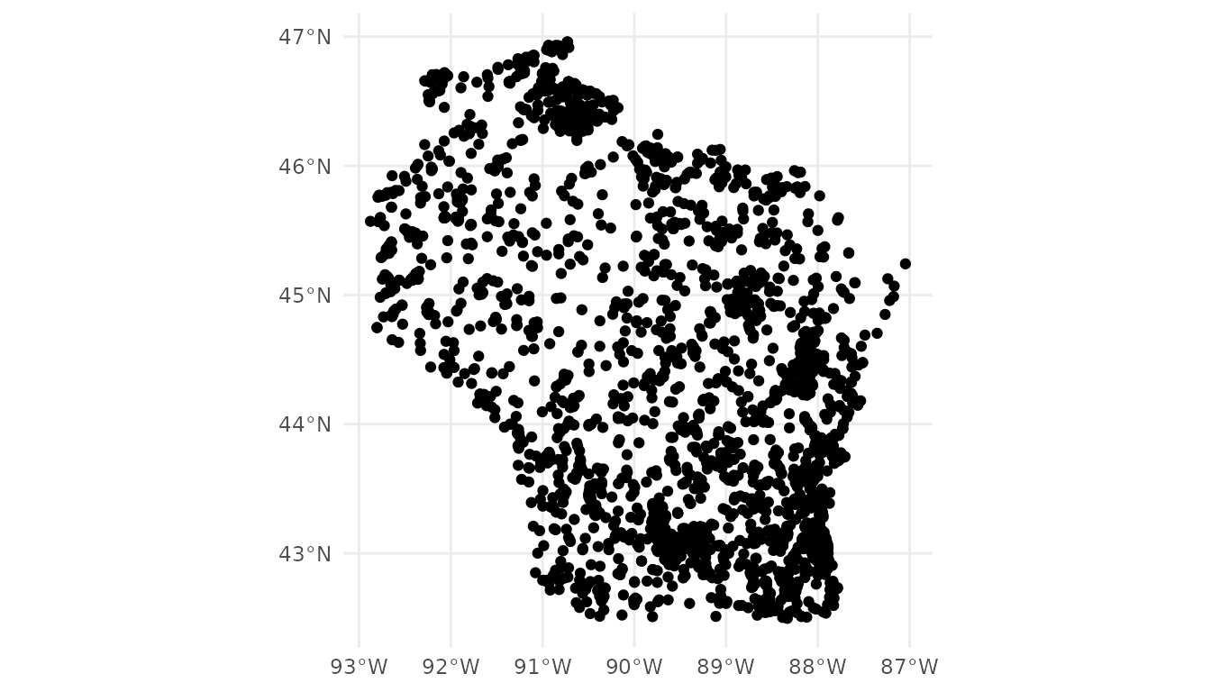
library(leaflet)

leaflet_crs <- "+proj=longlat +datum=WGS84" #default leaflet crs

leaflet(data = sites_wi |>
                sf::st_transform(crs = leaflet_crs)) |>
    addProviderTiles("CartoDB.Positron") |>
    addCircleMarkers(popup = ~monitoring_location_name,
                   radius = 0.1,
                   opacity = 1)
Time Series Metadata
The read_USGS_ts_meta function replaces the
whatNWISdata function.
Daily data and continuous measurements are grouped into time series, which represent a collection of observations of a single parameter, potentially aggregated using a standard statistic, at a single monitoring location. This endpoint provides metadata about those time series, including their operational thresholds, units of measurement, and when the earliest and most recent observations in a time series occurred.
To access these services on a web browser, go to https://api.waterdata.usgs.gov/ogcapi/v0/collections/time-series-metadata.
ts_available <- read_USGS_ts_meta(monitoring_location_id = "USGS-01491000",
                                  parameter_code = c("00060", "00010"))
The returning tables gives information on all available time series. For instance, we can pull a few columns out and see when each time series started, ended, or was last modified.
| parameter_name | statistic_id | begin | end | last_modified |
|---|---|---|---|---|
| Discharge | NA | 1948-01-14 | 2025-04-13 | 2025-04-13 |
| Temperature, water | 00011 | 2023-04-20 | 2025-06-06 | 2025-06-06 |
| Temperature, water | 00002 | 2023-04-22 | 2025-06-06 | 2025-06-06 |
| Discharge | 00003 | 1948-01-02 | 2025-06-06 | 2025-06-06 |
| Temperature, water | 00001 | 2023-04-22 | 2025-06-06 | 2025-06-06 |
| Temperature, water | 00003 | 2023-04-22 | 2025-06-06 | 2025-06-06 |
| Discharge | 00011 | 1985-10-01 | 2025-06-06 | 2025-06-06 |
| Temperature, water | 00001 | 1988-10-02 | 2012-05-10 | 2020-08-27 |
| Temperature, water | 00002 | 2010-10-02 | 2012-05-10 | 2020-08-27 |
| Temperature, water | 00003 | 2010-10-02 | 2012-05-10 | 2020-08-27 |
Daily Values
The read_USGS_daily function replaces the
readNWISdv function.
Daily data provide one data value to represent water conditions for the day. Throughout much of the history of the USGS, the primary water data available was daily data collected manually at the monitoring location once each day. With improved availability of computer storage and automated transmission of data, the daily data published today are generally a statistical summary or metric of the continuous data collected each day, such as the daily mean, minimum, or maximum value. Daily data are automatically calculated from the continuous data of the same parameter code and are described by parameter code and a statistic code. These data have also been referred to as “daily values” or “DV”.
To access these services on a web browser, go to https://api.waterdata.usgs.gov/ogcapi/v0/collections/daily.
library(dataRetrieval)

daily_modern <- read_USGS_daily(monitoring_location_id = "USGS-01491000",
                                parameter_code = c("00060", "00010"),
                                statistic_id = "00003",
                                time = c("2023-10-01", "2024-09-30"))
The first thing you might notice is that the new service serves data
in a “long” format, which means there is just a single observations per
row of the data frame (see: Pivot
Data). Many functions will be easier and more efficient to work with
a “long” data frame. For instance, here we can see how
ggplot2 can use the parameter_code column to create a
“facet” plot:
library(ggplot2)

ggplot(data = daily_modern) +
  geom_point(aes(x = time, y = value,
                 color = approval_status)) +
  facet_grid(parameter_code ~ ., scale = "free") +
  theme_bw()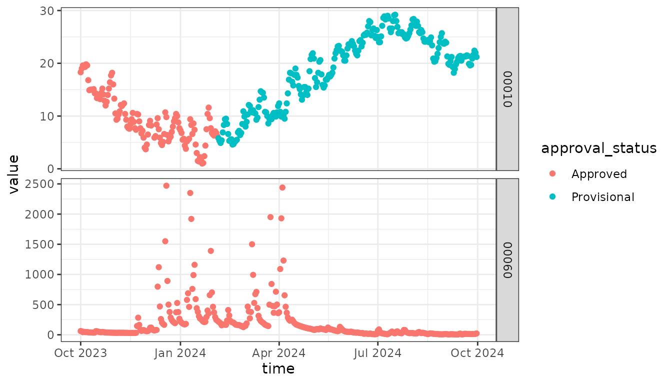
General Retrieval
The read_USGS_data function replaces the
readNWISdata function. This is a lower-level, generalized
function for querying any of the API endpoints.
The new APIs can handle complex requests. For those queries, users will need to construct their own request using Contextual Query Language (CQL2). There’s an excellent article https://api.waterdata.usgs.gov/docs/ogcapi/complex-queries/.
Let’s try to find sites in Wisconsin and Minnesota that have a drainage area greater than 1000 mi^2.
cql <- '{
  "op": "and",
  "args": [
    {
      "op": "in",
        "args": [
          { "property": "state_name" },
          [ "Wisconsin", "Minnesota" ]
        ]
    },
    {
      "op": ">",
        "args": [
          { "property": "drainage_area" },
          1000
        ]
    }
  ]
}'

sites_mn_wi <- read_USGS_data(service = "monitoring-locations",
                              CQL = cql)
Let’s see what that looks like:
leaflet_crs <- "+proj=longlat +datum=WGS84" #default leaflet crs

pal <- colorNumeric("viridis", sites_mn_wi$drainage_area)

leaflet(data = sites_mn_wi |>
                sf::st_transform(crs = leaflet_crs)) |>
    addProviderTiles("CartoDB.Positron") |>
    addCircleMarkers(popup = ~monitoring_location_name,
                     color = ~ pal(drainage_area),
                     radius = 0.1,
                     opacity = 1) |>
    addLegend(pal = pal,
              position = "bottomleft",
              title = "Drainage Area",
              values = ~drainage_area)
Discrete Samples
Discrete USGS water quality can be accessed via the
read_USGS_samples function. While this is a new, modern
USGS endpoint, it is not served in the same infrastructure as the rest
of these new advertised functions. See Samples Data) for information on
accessing USGS discrete water quality data.
Notes on dataRetrieval development
New Features
Style
New functions will use a “snake case”, such as
read_USGS_samples. Older functions use camel case, such as
readNWISdv. The difference is the underscore between words.
This should be a handy way to tell the difference between newer modern
data access, and the older traditional functions.
Structure
Historically, we allowed users to customize their queries via the
... argument structure. With ..., users needed
to know the exact names of query parameters before using the function.
Now, the new functions will include ALL possible
arguments that the web service APIs support. This will allow users to
use tab-autocompletes (available in RStudio and other IDEs).
Users will need to understand that they are not required to
specify all of these parameters. In fact, it is not advisable: the
systems can get bogged down with redundant query parameters. We
expect this will be easier for users, but it might take some time to
smooth out the documentation and test usability. There may be additional
consequences, such as users won’t be able to build up argument lists to
pass into the function.
Dependencies
Under the hood, dataRetrieval changed the dependency
from httr to httr2. httr2 is the
modern R package for web requests that is actively developed/maintained.
As we develop functions for the modern USGS web services, we’ll continue
to explore updating package dependencies. Since the new services offer
geospatial output, we also now require the sf package. The
whisker package was also included to help create POST CQL2
queries.
Developmental workflow
CRAN-stable documentation will be available on the GitHub pages: https://doi-usgs.github.io/dataRetrieval/
In-development documentation will be available on the USGS GitLab pages: https://water.code-pages.usgs.gov/dataRetrieval
Development of dataRetrieval will happen on a git branch
called “develop”. The “develop” branch will only move to the “main”
branch when we submit to CRAN, unless there are bug fixes that pertain
to the CRAN release. The “develop” branch WILL change frequently, and
there are no promises of future behavior. Users must accept that they
are using those functions at their own risk. If you willing to accept
this risk, the installation instructions are:
library(remotes)

install_github("DOI-USGS/dataRetrieval",
               ref = "develop")
HELP!
That’s a lot of new information and changes. There are certainly going to be scripts that have been passed down through the years that will start breaking once the NWIS servers are decommissioned.
Check back on the documentation often: https://doi-usgs.github.io/dataRetrieval/ Peruse the “Additional Articles”, when we find common issues people have with converting their old workflows, we will try to add articles to clarify new workflows.
Currently, you might be interested in:
If you have additional questions, email comptools@usgs.gov. General questions and bug reports can be reported here: https://github.com/DOI-USGS/dataRetrieval/issues