dataRetrieval Tutorial

This article will describe the R-package “dataRetrieval” which simplifies the process of finding and retrieving water data from the U.S. Geological Survey and other agencies.

Package Overview

dataRetrieval is available on Comprehensive R Archive Network (CRAN).

install.packages("dataRetrieval")

Once the dataRetrieval package has been installed, it needs to be loaded in order to use any of the functions:

library(dataRetrieval)

There are several vignettes included within the dataRetrieval package. The following command will open the main package introduction:

vignette("dataRetrieval", package = "dataRetrieval")

Additionally, each function has a help file. These can be accessed by typing a question mark, followed by the function name in the R console:

?read_waterdata_daily

Each function’s help file has working examples to demonstrate the usage. The examples may have comments “## Not run”. These examples CAN be run, they just are not run by the CRAN maintainers due to the external service calls.

Finally, if there are still questions that the vignette and help files don’t answer, please post an issue on the dataRetrieval GitHub page:

https://github.com/DOI-USGS/dataRetrieval/issues

For a longer introduction to the dataRetrieval package, see:

https://rconnect.usgs.gov/dataRetrieval_workshop

Orientation

dataRetrieval provides US water data mainly via 3 sources:

National Water Information System (NWIS)
Water Quality Portal (WQP)
USGS APIs (USGS), which are new or in-development .

Functions in dataRetrieval look like readNWISdv, readNWISuv, readWQPqw, whatNWISdata, etc. What does that mean? The functions are generally structured with a prefix, middle, and suffix:

Prefix: “read” or “what”
- “read” will access full data sets
- “what” will access data availability
Middle: “NWIS”, “USGS”, “WQP”:
- NWIS functions get data from legacy NWIS web services.
- USGS functions are the functions that will eventually replace the legacy NWIS functions. These pull from modern USGS API services.
- WQP functions are for discrete water-quality data from the Water Quality Portal.
Suffix: “data” or other:
- Functions that end in “data”: These are flexible, powerful functions that allow complex user queries.
- Functions that don’t end with “data” are user-friendly functions that assume site, code, and start/end dates are known.

Data Overview

There are many types of data served from NWIS. To understand how the services are separated, it’s helpful to understand that each data type is retrieved from a completely different web service or API.

NWIS has traditionally been the source for all USGS water data
Legacy NWIS services will be retired (scheduled 2026, but uncertain):
- https://waterdata.usgs.gov/blog/nwisweb-decommission-summary/
USGS functions will slowly replace NWIS functions
- read_waterdata_samples has replaced readNWISqw
- read_waterdata_daily can replace readNWISdv
- read_waterdata_monitoring_location can replace readNWISsite
- read_waterdata_ts_meta can replace whatNWISdata
Discrete water quality data:
- WQP functions should be used when accessing non-USGS discrete water quality data
- read_waterdata_samples should be used for USGS data

NWIS Data: Current NWIS offerings

data_type_cd	Function	Data description	Replacement Function
uv	readNWISuv	Continuous data	None yet
dv	readNWISdv	Daily aggregated	read_waterdata_daily
gwlevels	readNWISgwl	Groundwater levels	None yet
site	readNWISsite	Site metadata	read_waterdata_monitoring_location
pcode	readNWISpCode	Parameter code metadata	None yet
stat	readNWISstat	Site statistics	None yet
rating	readNWISrating	Rating curves	None yet
peak	readNWISpeak	Peak flow	None yet
use	readNWISuse	Water Use	None yet
meas	readNWISmeas	Discrete surface water	None yet
	readNWISdata	General data import for NWIS	read_waterdata

USGS Basic Retrievals

The USGS uses various codes for basic retrievals. These codes can have leading zeros, therefore they need to be a character (“01234567”).

Site ID (often 8 or 15-digits)
Parameter Code (5 digits)
- Full list: readNWISpCode("all")
Statistic Code (for daily values)
- Full list:
- http://help.waterdata.usgs.gov/code/stat_cd_nm_query?stat_nm_cd=%25&fmt=html/

Here are some examples of a few common parameter codes:

Parameter Codes	Short Name
00060	Discharge
00065	Gage Height
00010	Temperature
00400	pH

Statistic Codes	Short Name
00001	Maximum
00002	Minimum
00003	Mean
00008	Median

Use the readNWISpCode function to get information on USGS parameter codes. You can use “all” to get a full list. Then use your favorite data analysis methods to pull out what you need. Here is one example to find all the phosphorous parameter codes:

pcode <- readNWISpCode("all")

phosCds <- pcode[grep("phosphorus",
  pcode$parameter_nm,
  ignore.case = TRUE
), ]

Explore the wide variety of parameters that contain “phosphorus” in the parameter_nm:

User-friendly retrievals: NWIS

Sometimes, you know exactly what you want. If you know:

The type of data (groundwater, unit values, daily values, etc..)
USGS site number(s)
USGS parameter code(s)
Time frame (start and end date)

You can use the “user-friendly” functions. These functions take the same 4 inputs (sites, parameter codes, start date, end date), and deliver data from the different NWIS services.

Pheasant Branch Creek Example

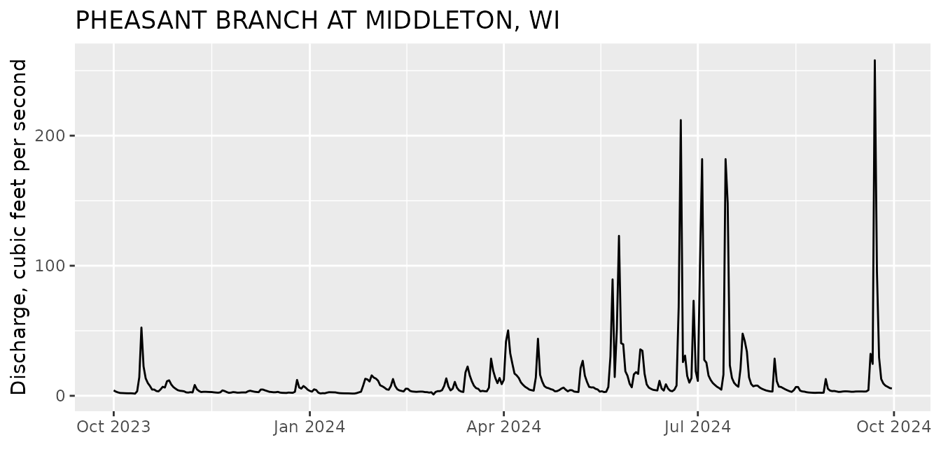
Let’s start by asking for discharge (parameter code = 00060) at a site right next to the old USGS office in Wisconsin (Pheasant Branch Creek).

siteNo <- "USGS-05427948"
pCode <- "00060"
start.date <- "2023-10-01"
end.date <- "2024-09-30"

pheasant <- read_waterdata_daily(monitoring_location_id = siteNo,
                            parameter_code = pCode,
                            time = c(start.date, end.date))

From the Pheasant Creek example, let’s look at the data. The column names are:

names(pheasant)

##  [1] "daily_id"               "statistic_id"           "monitoring_location_id"
##  [4] "time"                   "unit_of_measure"        "time_series_id"        
##  [7] "parameter_code"         "value"                  "approval_status"       
## [10] "last_modified"          "qualifier"              "geometry"

Let’s make a simple plot to see the data:

library(ggplot2)
ts <- ggplot(
  data = pheasant,
  aes(time, value)) +
  geom_line()
ts

Then we can use the readNWISpCode and read_waterdata_monitoring_location functions to create better labels:

parameterInfo <- readNWISpCode(pCode)
siteInfo <- read_waterdata_monitoring_location(siteNo)

ts <- ts +
  xlab("") +
  ylab(parameterInfo$parameter_nm) +
  ggtitle(siteInfo$monitoring_location_name)
ts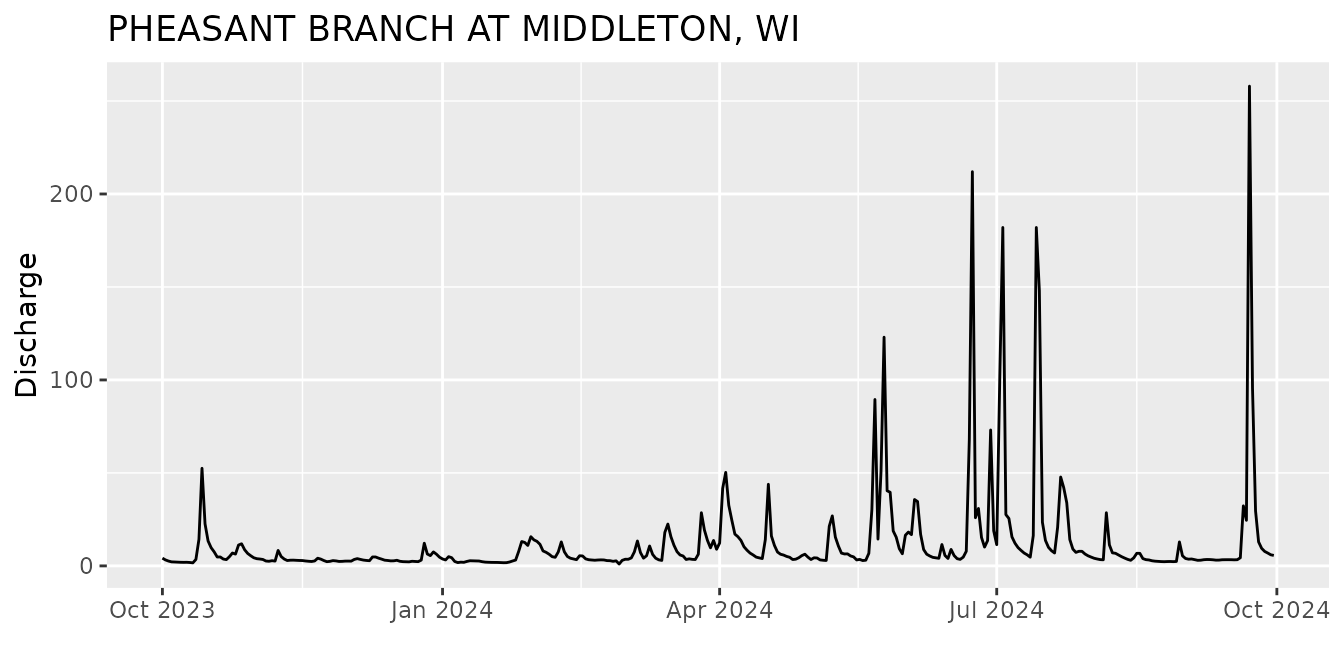

Known USGS site, unknown service/pcode

The most common question the dataRetrieval team gets is:

“I KNOW this site has data but it’s not coming out of dataRetrieval! Where’s my data?”

First verify that the data you think is available is actually associated with the location. For time series data, use the read_NWIS_ts_meta function to find out the available time series data.

library(dplyr)

site <- "USGS-05407000"
ts_data_available <- read_waterdata_ts_meta(monitoring_location_id = site) 


data_available <- ts_data_available |> 
  sf::st_drop_geometry() |> 
  mutate(begin = as.Date(begin),
         end = as.Date(end)) |> 
  select(parameter_name, parameter_code, statistic_id, computation_identifier,
         begin, end)

The time series that have “Instantaneous” in the computation_identifier column will be available in the instantaneous data service (currently readNWISuv), and the rest of the data will be available in the daily service (read_waterdata_daily).

dv_pcodes <- data_available$parameter_code[data_available$computation_identifier != "Instantaneous"]
stat_cds <- data_available$statistic_id[data_available$computation_identifier != "Instantaneous"]

dv_data <- read_waterdata_daily(monitoring_location_id = site,
                           parameter_code = unique(dv_pcodes),
                           statistic_id = unique(stat_cds))

uv_pcodes <- data_available$parameter_code[data_available$computation_identifier == "Instantaneous"]

uv_data <- readNWISuv(siteNumbers = gsub("USGS-", "", site),
                      parameterCd = unique(uv_pcodes))

peak_data <- readNWISpeak(gsub("USGS-", "", site))

For discrete water quality data, use the summarize_waterdata_samples function:

discrete_data_available_all <- summarize_waterdata_samples(site) 

discrete_data_available <- discrete_data_available_all |> 
  select(parameter_name = characteristicUserSupplied, 
         begin = firstActivity, end = mostRecentActivity,
         count = resultCount)

The discrete water quality data can be accessed with the read_waterdata_samples function:

samples_data <- read_waterdata_samples(monitoringLocationIdentifier = site, 
                                  dataProfile = "basicphyschem")

Water Quality Portal (WQP)

dataRetrieval also allows users to access data from the Water Quality Portal. The WQP houses data from multiple agencies; while USGS data comes from the NWIS database, EPA data comes from the STORET database (this includes many state, tribal, NGO, and academic groups). The WQP brings data from all these organizations together and provides it in a single format that has a more verbose output than NWIS.

This tutorial will use the modern WQX3 format. This is still considered “beta”, but it is the best way to get up-to-date multi-agency data.

The single user-friendly function is readWQPqw. This function will take a site or vector of sites in the first argument “siteNumbers”. USGS sites need to add “USGS-” before the site number.

The 2nd argument “parameterCd”. Although it is called “parameterCd”, it can take EITHER a USGS 5-digit parameter code OR a characterisitc name (this is what non-USGS databases use). Leaving “parameterCd” as empty quotes will return all data for a site.

So we could get all the water quality data for site USGS-05407000 like this:

qw_data_all <- readWQPqw(siteNumbers = site,
                         parameterCd = "", 
                         legacy = FALSE)

or 1 parameter code:

qw_data_00095 <- readWQPqw(siteNumbers = site,
                           parameterCd = "00095", 
                           legacy = FALSE)

or 1 characteristic name:

qw_data_sp <- readWQPqw(siteNumbers = site,
                        parameterCd = "Specific conductance", 
                        legacy = FALSE)

Discover Data

This is all great when you know your site numbers. What do you do when you don’t?

There are 2 dataRetrieval functions that help with USGS data discovery:

read_waterdata_monitoring_location finds sites within a specified filter
read_waterdata_ts_meta summarizes the time series meta data

And 2 functions that help with discover in WQP:

readWQPsummary summarizes the data available within the WQP by year.
whatWQPdata summarizes the data available within the WQP.

Available geographic filters are individual site(s), a single state, a bounding box, or a HUC (hydrologic unit code). See examples for those services by looking at the help page for the readNWISdata and readWQPdata functions:

Here are a few examples:

Time/Time zone discussion

The arguments for all dataRetrieval functions concerning dates (startDate, endDate) can be R Date objects, or character strings, as long as the string is in the form “YYYY-MM-DD”.
For functions that include a date and time, dataRetrieval will take that information and create a column that is a POSIXct type. By default, this date/time POSIXct column is converted to “UTC”. In R, one vector (or column in a data frame) can only have ONE timezone attribute.
- Sometimes in a single state, some sites will acknowledge daylight savings and some don’t
- dataRetrieval queries could easily span multiple timezones (or switching between daylight savings and regular time)
The user can specify a single timezone to override UTC. The allowable tz arguments are OlsonNames (see also the help file for readNWISuv).

Large Data Requests

It is increasingly common for R users to be interested in large-scale dataRetrieval analysis. You can use a loop of either state codes (stateCd$STATE) or HUCs to make large requests. BUT without careful planning, those requests could be too large to complete. Here are a few tips to make those queries manageable:

Please do NOT use multi-thread processes and simultaneously request hundreds or thousands of queries.
Take advantage of the whatWQPdata and whatNWISdata functions to filter out sites you don’t need before requesting the data. Use what you can from these faster requests to filter the full data request as much as possible.
Think about using tryCatch, saving the data after each iteration of the loop, and/or using a make-like data pipeline (for example, see the drake package). This way if a single query fails, you do not need to start over.
The WQP doesn’t always perform that well when there are a lot of filtering arguments in the request. Even though those filters would reduce the amount of data needed to transfer, that sometimes causes the pre-processing of the request to take so long that it times-out before returning any data. It’s a bit counterintuitive, but if you are having trouble getting your large requests to complete, remove arguments such as Sample Media, Site Type, these are things that can be filtered in a post-processing script. Another example: sometimes it is slower and error-prone requesting data year-by-year instead of requesting the entire period of record.
Pick a single state/HUC/bbox to practice your data retrievals before looping through larger sets, and optimize ahead of time as much as possible.

There are two examples scripting and pipeline that go into more detail.

But wait, there’s more!

There are two services that also have functions in dataRetrieval, the National Groundwater Monitoring Network (NGWMN) and Network Linked Data Index (NLDI). These functions are not as mature as the WQP and NWIS functions. A future blog post will bring together these functions.

National Groundwater Monitoring Network (NGWMN)

Similar to WQP, the NGWMN brings groundwater data from multiple sources into a single location. There are currently a few dataRetrieval functions included:

Network Linked Data Index (NLDI)

The NLDI provides a information backbone to navigate the NHDPlusV2 network and discover features indexed to the network. For an overview of the NLDI, see: https://rconnect.usgs.gov/dataRetrieval/articles/nldi.html

Laura DeCicco

June 18, 2025